If you have work with some kind of industrial or marine automation, then most probably you've heard before the term PID. PID controllers are very common in closed-loop systems today. Here is how this system can calculate and minimize the error with great precision.
History
The whole story began as a marine application, when people were trying to find ways to make reliable and accurate ship steering systems. But the problem was that, if the automation turns the rudder let's say left, the ship will not turn instantaneously, instead it needs a long course, for ships do not steer like like cars, instead they have a big hysteresis. Another problem is also that when the ship finally turns to the right direction and the automation turns the rudder straight, the ship keeps turning left due to inertia and many other parameters like waves, wind, speed etc.
At first, proportional systems were developed to do this. A proportional systems reads the feedback (electronic compass) and turns the rudder according to the angle that the ship needs to turn. If for example the ship had to turn 45 degrees left, the rudder would turn 20 degrees, and as the ship slowly turns to this direction, the rudder decreases its angle proportionally. But this system has a great disadvantage: Either the rudder will oscillate left and right because the ship will never stay on course precisely due to external disturbances, or the system will stabilize with a small constant error in angle.
Elmer Sperry was the first to introduce an early PID-type controller back in 1911, and it took another 11 years until engineer Nicolas Minorsky published the first theoretical analysis of a PID controller (Minorsky 1922). In order to design an automatic steering system for the US navy, Minorsky spent several hours observing helmsmen while on duty. He noticed that the helmsman turned the rudder not only according to the current error, but also according to the past errors and the rate of change. During first trials with a PI controller on the USS New Mexico, the system achieved an error of 2 degrees. When the parameter D was added (PID) the system managed to achieve error of 1/6 of a degree, better than most helmsmen could achieve.
What is P, what is I, what is D?
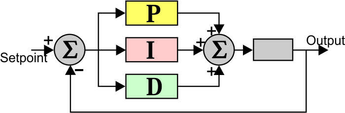
The word PID is composed by the first letters from the terms Proportional, Integral and Derivative. The Proportional, Integral, and Derivative terms are summed to calculate the output of the PID. Here is the diagram to get a first (just a first) idea how this system works:
As you see, the setpoint is compared with the feedback. With the error (setpoint-feedback) the controller calculates the three terms (P-I-D), and finally these terms are added to calculate the new output.
Before i go into details, i need to define some terms in advance:
Error [e]: The error is the difference between the target position and the real position. Suppose for example that we have a system that controls the temperature. If the set-point is 100oC and the actual temperature is 60oC, then the error is 40oC. The error is represented by the letter "e".
Proportional gain parameter [Kp]: This is a number that controls the proportional term. In a real life controller, this number is usually a controller parameter which the end-user can change
Integral gain parameter [Ki]: This is a number that controls the integral term. In a real life controller, this number is usually a controller parameter which the end-user can change
Derivative gain parameter [Kd]: This is a number that controls the derivative term. In a real life controller, this number is usually a controller parameter which the end-user can change
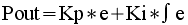
The term P: Proportional
The proportional term changes the output according to the error. A simple proportional controller has only one control parameter, the Kp. By changing this parameter, the controller becomes more or less reactive in changes. The proportional term is given by this form:
P = Kp x e
And the output of the controller:
Pout = P = Kp x e
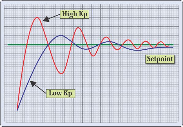
The higher the Kp parameter, the faster the system will try to reach the set-point, but also high proportional gain turns the system unstable and it oscillates around the set-point. On the other hand, if the Kp is low, then the the system will stabilize with a constant error bellow (or above) the set-point, because the output will not provide sufficient power for the system to reach the final position. Here is a graph to better understand this parameter:
The red line shows the response of the system with a high Kp. The system will try to reach the set-point faster, but the overshoot is high as well as the error. This drives the system into an unstable state in which it oscillates around the set-point. The blue line shows the response with a low Kp. The system will reach the set-point slower and it will cause a much smaller overshoot. But after a few oscillations, the controller output does not provide enough power to change the system, thus it will remain stable a little bellow the set-point.
The term I: Integral
A proportional system is usually not sufficient to eliminate the error. The system must not only change its output according to the current error, but it must also be able to watch and change the output according to the past errors. The integral is the sum of the errors over time. What this means is that, if the error is big, then the integral builds up as time passes and the output changes rapidly to eliminate the error.
Now suppose that we have the same example as before, a proportional system that has a low Kp. First of all, the system will respond much faster at the beginning, because the error will build up a big integral. Then, when the system is stabilized little bellow the set-point, the integral will take over. This small error is added over time to increase the integral, and finally it will change the system's output. Finally, the system will stabilize onto the set-point.
Like before, the integral term is multiplied by the integral gain parameter to increase or decrease the effect and it is given by this form:
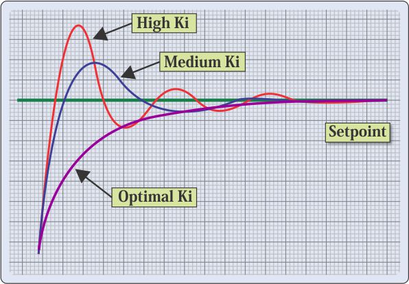
Now, suppose that we have a proportional system with low Kp and an integral term. Such a system is named PI, and here is how the system reacts as Ki changes:
A high integral gain (Ki) (red line) causes a faster system response, but also causes overshoot. Unlike the pure proportional system, despite the overshoot, the system is not driven into an unstable state. After a few oscillations the system will stabilize on the set-point. As the integral gain gets smaller (blue line), the system responses slower, but it stabilizes much faster with less oscillations. The optimal integral gain (purple line) causes the system to respond very slow but it stabilizes on the set-point with almost no oscillations.
A PI system output is mathematically represented as:
In other words, the output is the sum of the Proportional term plus the Integral term.
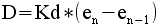
The term D: Derivative
The third and last term is the Derivative. This term calculates the rate of change of the error and adds to the output accordingly. If the error changes slow, then the derivative is increased in order to make the PID system respond faster. On the other hand, if the error is changes rapidly, the derivative is decreased in order to make the system more stable and avoid oscillations. The formula to describe the derivative is:
The output of a full PID controller is given my this mathematical form:
@Saimul If there is no oscillation then maybe you don't need a PID controller. Does it get unstable if you increase Kp too much? Is there a steady-state error?
I'm also trying build PID controller to control temperature of heater. Heater heat the metal plate.
Till this time:
Heater is about 500W, and i trying control temperature by the triac. Heater is less frequently ON, if temperature is closer to the temperature that we want to achieve (set to 100deg.C). In this algorithm heater is on in duty from 10% do 100%. The best result is when:
- duty=100% for T<70deg.C
- duty=80% for T=71 to 80deg.C
- duty=60% for T=81 to 90deg.C
- duty=50% for T=91 to 100deg.C
- when T>=100deg.C then heater is OFF
In algorithm above temperature oscillates in about /- 3deg.C
And that way I would like to implement PID controller.
So for example if sum from calculating PID will be lets say from -50 to 120 then for my duty from 0 to 100% i must convert PID to range 0-100 so:
PID=-50 to 120
DUTY=PID 50
DUTY=0 to 170
DUTY=DUTY/1.7
Is that correct translation ?
At 13 February 2014, 13:45:08 user Saimul wrote: [reply @ Saimul]
Hi...I am working with a development of PID controller for a water heater. The problem that I am facing right now in determining the value of Kp,Ki and Kd. If I want to use Ziegler-Nicholas method for tuning PID then I have to determine the critical gain Kc and oscillation period Pc. After I can calculate PID parameters accordingly. But the problem is there is no oscillation in my system. So what should I do now?
@sierra It largely depends on your application. If you have an 8-bit then you have to limit it from 0 to 255, or if you need negative numbers you limit to 127. So you have to do the proper divisions when you read the input to fit these ranges. Which means that you have to know before hands the minimum and maximum values that the sensor will send you
At 13 November 2013, 16:53:09 user sierra wrote: [reply @ sierra]
Hi,
Nice work, thank you.
When you calculate the P_Out value it may be too large or too small (negative). In such a case you may have to limit the maximum P_Out value. How do you determine the minimum and maximum P_Out value.
@Pushkin2023 fot Ti and Td i'd say the faster the better, depending on the response of the system (you want very quick response). As for the D term, do not reset it to zero, it will reset itself in a couple of Td times...
Very nice tutorial. I'm trying to make a pid controller for my rotary inverted pendulum. I'm doing the pid computing every 20ms (timer2 interrupt, sets a flag in main loop), how should be Ti and Td?(how many times greater then pid loop) Another thing: the d_term and i_term shouldn't be reseted to 0 when the error is 0 or very very close to 0 ?
Morning
Thank you very much
I was wondering how to adjust the set point and can I program it using flowcode mplab from microchip? If not what ic and program should I use ?
@NOAK an 8-bit number can measure from 0 to 255 with integer numbers. So, it fully covers the range 0 to 100. But it cannot measure from 0 to 600 with 1 degree accuracy... Maybe with 3 degrees accuracy (because 3*256=768)
At 24 August 2012, 11:12:34 user NOAK wrote: [reply @ NOAK]
"For example, a temperature controller that is used for a system which measures temperatures from 0 to 100 degrees with 1oC accuracy can be implemented with 8-bit registers, But if the system measures from 0 to 600oC then the 8-bits are just not enough."
could u explain why 8-bit MCU is not enough for 0-600 C application?
for example , i want to control a servo motor to move it to a commanded position and the output of the control system is PWM . so i should select proper P,I & D values so that the summation , i.e PID , is the correct PWM output which makes the motor move to the commanded position regardless to what degree the PWM should be propotional to the PID vlaue .
@akshay That is the idea. You make all these calculations to come up with an output power that is required. This output can b anything, like an analog voltage, an angle of a servomotor, a throttle position of an engine.... anything.
@akshay now this depends on the control circuit. If it is PWM for example, you can change the duty cycle depending on the value you calculate... e.g. 0-100% duty cycle = 0 - 500 calculated PID
Or if it has an analog output... you can change the analog value...
... it is 8 pages long! Filled with in-depth description and pictures the developmental changes to his code. And it is linked to the Arduino Playground code library, along with an Autotune library, at:
http://arduino.cc/playground/Main/LibraryList
in the Input / Output subcategory.
Finally, the author links to the site of his own mentor, at:
http://controlguru.com/
I have not yet looked at this myself, but I hope to find it educational.
@Artur the idea of the It and Dt time parameters, is to avoid an overflow. The I parameter for example is used to have usually small changes, so that the operator can balance the immediate changes of the P parameter. If the I builds up on every cycle, then it will become huge very fast, and the system will not become stable. The idea is that the I build up slowly, and the system becomes stable slowly. The delay depends on the system's response. If a systems responses fast (for example hot air blower) then the It is small, otherwise (eg large water tank heater) It may be very large. Same stands for D.
The parameter P follows the changes in output, it reads the error and changes the power accordingly in every cycle. The parameter I builds up slowly. Here is how we use to explain these parameters.
P is the present, it looks at the output and changes with the present error.
I is the past, it looks at the past errors and changes accordingly.
D is the future, every Dt it looks at the error and according to the rate of change it tries to predict the future
I am not sure what the result of the ring buffer would be. It sounds as a good idea, since the errors some 100 cycles before (for example) are not important for the I term. If i make another PID controller, i will experiment with this idea.
At 26 January 2012, 21:34:05 user Artur wrote: [reply @ Artur]
I agree with others: best explanation I've seen so far. I'm wondering, would it be a good idea to store error in a ring buffer, e.g. 16 last values and calculate I and D from that on every iteration? If not then why. Other than the obvious added CPU cost.This way I would follow changes in output, not change incrementally every Ti cycles. Also why not calculate D in every loop based on previous loop's error?
@Bill Kostelidis regarding the Integral, if you calculate it in every cycle, the system will never be stable, unless the system is highly reactive. That is exactly the point of the integral term existence after all: to check the progress between time intervals and decide if needs more or less power.
To use the result of the PID, you need first to scale it to an easy-usable number. I use for example -127 to +127 which is one byte. The, you can either translate the number to 0-256 or just use it as is. Finally, you need to have a variable output. If the output is for example PWM, then i would translate the PID result to 0-256. Then, i would use this number as a PID duty cycle (0-0% 256=100%).
I really like your projects. Although I have my disagreements with the way that the Integral is not calculated in every circle, since it is working, you must be correct!
I am working in a PID project myself and I have a question, if you can help, it's great.
I am heating water with immersion heaters, resistors. They are plugged directly in 220 Volts but I will use PWM to control them. The control is going to come from my PID.
After I get the output from my PID controller, how am I going to translate it to PWM? I mean, if the output of my PID indicates 2 Celsius degrees down, how am I going to say to my PWM to adjust to 2 degrees down?
I am going to work experimentally at first, but I am searching to find a more solid solution, any ideas?
Thanks,
Bill.
At 27 October 2011, 4:01:13 user sorin wrote: [reply @ sorin]
I am a Vietnamese. I have read many textbooks about PID control in some subjects in university, but I've never really understood the meaning of this method, I think the theory is explained too complicatedly than what it really means.
This post is a great explanation! I understood it easy.
Thank you very much!
At 30 September 2011, 16:20:54 user Erik T wrote: [reply @ Erik T]
This IS the best explanation of PID I have ever seen.
The historical background adds so much to the explanation,
that it makes so much more sense.
I'd like to know how you created the graphs!
I think a graphical demonstration program of PID would be awesome.
It could allow users to set parameters and watch and compare settings.
It could then show how to tune PID, using either method or both.
I have retuned repaired PID controllers for CNC equipment, and until
now have never understood why the directions for tuning were what they
were. "... then reduce these two levels, and then turn this third one up until the machine oscillates." It all makes sense now.
thank you, I look forward to coding something like the demo program
because I cannot find one.

 Home
Home
 Projects
 Experiments
 Circuits
 Theory
 BLOG
BLOG
 PIC Tutorials
 Time for Science


 Contact
 Forum
Forum
 RSS
RSS


 Reddit this